What is the difference between a z-test and a t-test?

Randomly pick four numbers between -48 and +48 and take their mean. There are lots of different combination that could give me a mean of zero, but to get a mean of 48, I’d have to pick four 48s in a row; a highly unlikely combination! The same goes for -48. If I ask a computer to try doing this 10,000 times, and plot a histogram of the mean I get each time, here’s how it looks:

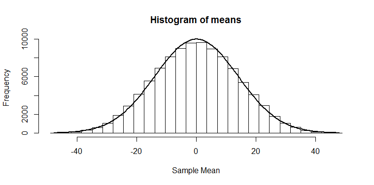
So, you’re possibly familiar with this: the Central Limit Theorem tells us that when we take the mean of a bunch of random numbers, that mean will end up being (roughly!) normally distributed. Furthermore, it tells us that the standard deviation of this normal distribution will be where is the standard deviation of the numbers we started with and is the size of our sample. In our case, the standard deviation of the numbers -48 through 48 (if chosen with equal probability) is 28:

.

Our sample size is 4,

,

so the standard deviation of the above normal distribution should be , which looks about right for the above histogram!

Now, if we divide by this “standard error” (the standard deviation of our means), we should have numbers that are normally distributed with mean 0 and standard deviation of 1. We have -scores:

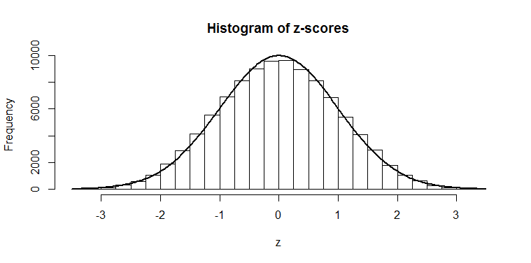
And we can compare these numbers to the numbers in our z-tables in our statistics books. We can see that, for example, getting a mean of 28 or more has only a 2.5% probability — because it has a z-score of . This also agrees with the histogram of means, where we can see there were not very many cases above 28. This is a -test, and we run a -test when we know what the true standard deviation of the population is.

What if we have a set of numbers that we are taking the mean of, but we don’t know what the population standard deviation is? Well, we could use the standard deviation of our sample as a reasonable guess at the standard deviation of the population. But since that’s just a guess, we don’t get quite the numbers we would have had before, and we end up with a slightly different shape of histogram:

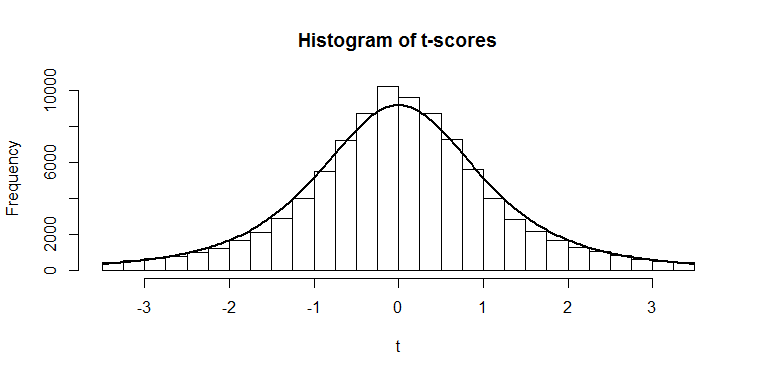
The black line that I’ve fitted to this histogram is the -distribution with three degrees of freedom. (Three because degrees of freedom is ). You can see it is fatter at the edges; we saw that there was only a 2.5% chance of getting a -score of 2 or more, but there is a 7% chance of getting a -score of 2 or more in this case. So, if we don’t know what the true population standard deviation is, we can use our sample standard deviation as an estimate, but we need to compare it against a different distribution (the -distribution), which means looking at a different table in the back of your statistics book (a table referring to ““), and we call it a “-test”.

If you’re curious where the shape of this distribution comes from, my next post should give you a pretty good idea of it.