In my last post, I talked about how sample means tend to be normally distributed, but if we divide them by their sample standard deviation they are t-distributed. That post was really written as a supporting post for this one, and I’ll assume that you have read that post or understand these things already. Here I’ll show you a little experiment that will give you a pretty good idea of exactly how the 
So, we’re using our sample standard deviation as an estimate of the population standard deviation. What we get then isn’t normally distributed any more because the sample standard deviation will come out different for every sample we pick:
Sometimes it will be a bit too high, which will mean we’ll be dividing our mean by a standard deviation that is too large, and our “
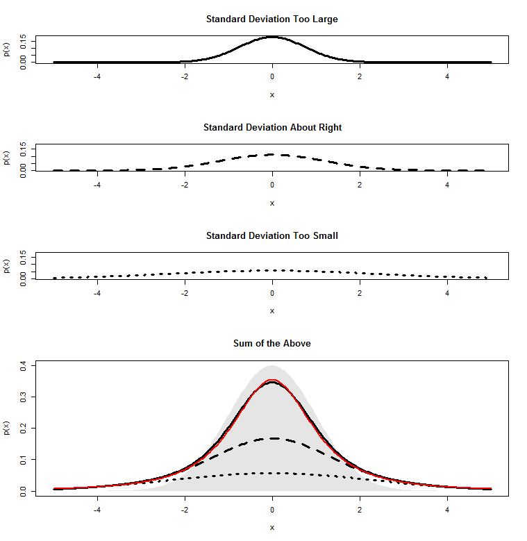
Since a distribution is like a “pile” of probability mass for any given score, we can combine all these possibilities by piling each pile on top of the other, and this is what I have done in the bottom graph above. The thick black line represents the top of the pile, the sum of all three of our normal distributions. The red line is a
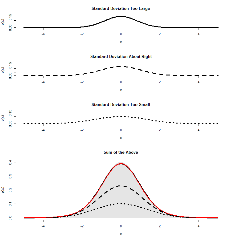
At the bottom I’ve copied my R code for generating the above plots, in case you’d like to play with it. If we increase our degrees of freedom, for example, by changing to df=10, we can see why the
Since we’re adding up a bunch of normal distributions that all look very similar, it’s no surprise that what we get at the end is something that looks like a normal distribution: the thick black and red lines both match the grey shaded normal distribution pretty closely.
The goal of this post is to show you that a t-distribution is just a pile of different normal distributions with different spreads. And, in fact, one way to derive the shape of the t-distribution is to add up the infinite number of different normal distributions that we could get for every different “wrong” standard deviation that we could get.
Here’s the code:
# tweak the degrees of freedom here

df = 2
# you can tweak this number if you want to explore non-central t-distributions
# the approximation I'm using falls apart a bit for very large ncp (>2), though
ncp = 0
# get standard errors that are too small, about right and too large
plotnames = c("Standard Deviation Too Small", "Standard Deviation About Right", "Standard Deviation Too Large")
SEs = sqrt(qchisq(c(1,3,5)/6,df)/df)
# plot the individual normal distributions
layout(c(1,2,3,4,4))
xs = seq(-5,5,length.out=300)
plots = sapply(SEs,function(SE)dnorm(xs,mean=ncp/SE,sd=1/SE)/3)
sapply(3:1,function(n)plot(xs,plots[,n],type="l",lwd=3,lty=4-n,ylim=c(0,max(plots)),xlab="x",ylab="p(x)",main=plotnames[n]))
# plot these normal distributions piled on top of each other
stackedplots = apply(plots,1,cumsum)
matplot(xs,t(stackedplots),type="l",lwd=3,col="black",ylim=c(0,dnorm(0)),xlab="x",ylab="p(x)",main="Sum of the Above",lty=3:1)
polygon(xs,dnorm(xs,ncp),col=rgb(0,0,0,.1),border=NA)
lines(xs,dt(xs,df,ncp),col="red",lwd=2)