Wilks’ Theorem: Why do likelihood ratio tests work?

This is a question I’ve wanted to understand for quite some time. The likelihood ratio test seems to be almost a silver bullet for many of the modern maximum-likelihood approaches to statistics, but it always seemed quite mysterious to me that -2 \mathrm{log}p(x;\theta) should have a known distribution. I’ve spent my morning today working through a few derivations for this, and it’s some dense stuff! I haven’t yet looked at the full multi-dimensional proofs, so I am no expert by any means, but I have managed to get my head around the proof of a simplified Wilks’ theorem here, and what follows is a little summary of this, partly for my own reference, and partly because I’d have found a simple overview helpful before I looked at the proper proofs, so I hope it might be helpful someone else too. Clearly, I’m no expert on this particular topic, and I’d welcome any corrections or suggested improvements.

If you don’t know what a likelihood ratio test is, or what maximum likelihood is, I refer you to Google! There is plenty of stuff out there on what they are and how they are run. What I found harder to find, however, was anything offering a simple, crude intuition of why it works. So, I thought, now that I have my head around a simple version of the derivation, it might be nice to make a quick, simple graphical summary. I gloss over a lot of technical details about different types of convergence etc here. This is just the bare bones.

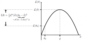
To keep the maths as simple as possible, I’ll use quite a bit of loose/abusive notation; and \mathcal{L} will refer to the log likelihood, \mathcal{L}(\theta)=\mathrm{log}p(x;\theta). The whole derivation is based on simple Taylor expansions around either the maximum likelihood parameter estimate \hat\theta or the (null hypothesis) true parameter \theta_0. This seems sensible, as these two should be relatively close to each other. To keep things simple, I will discuss as if the log likelihood \mathcal{L}(\theta) were quadratic — which, by our expansions, we are assuming to be true locally, anyway. (And for a normal distribution, this will not be an approximation; another beautiful thing about the normal distribution is that the log likelihood is a quadratic!). Here, then, is a plot of \mathcal{L}(\theta):

likelihood ratio test fig 1

The gap between the dashed lines represents the log likelihood ratio `LR’, and we are using here a Taylor expansion to find this difference in log values (i.e. log of a ratio). Bear in mind that \mathcal{L}'(\hat\theta)=0 since we are at a maximum on the likelihood surface; this is why there is no linear term in our expansion. The key to the proof is the claim in the underbrace, that \hat\theta will be normally distributed around \theta_0, with variance of \mathrm{Var}(\hat\theta)=-1/\mathbb{E}(\mathcal{L}''). If we can prove that this is true, then we are done: it is clear, in this case that -2\mathrm{LR}\sim\chi^2(1). Though, that does assume that the curvature in the log likelihood surface for our data \mathcal{L}'' is close to its expectation.

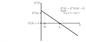
To see that it is indeed distributed like this, take a look at the derivative of the above graph:

likelihood ratio test fig 2

Since we now have a straight line, then if we can show that \mathcal{L}'(\theta) is normally distributed, then so too should be (\hat\theta - \theta_0). And, indeed, the log likelihood is found by summing the log likelihoods across all datapoints, each of which is i.i.d., so central limit theorem gives us that it is (asymptotically) normally distributed, and so too should be its derivative \mathcal{L}'(\theta;\mathbf{x})=\sum_i \mathcal{L}'(\theta;x_i).

The sampling variance of the likelihood derivative \mathcal{L}_i'=\mathcal{L}'(\theta;x_i) for a given datapoint is known as the Fisher information, and there is a nice clean, simple proof that \mathrm{Var}(\mathcal{L}'_i)=-\mathbb{E}(\mathcal{L}_i'') here on Wikipedia. Since our overall likelihood is just a sum \mathcal{L'}=\sum_i\mathcal{L'}_i, then

\mathrm{Var}(\mathcal{L}')=\sum_i\mathrm{Var}(\mathcal{L}'_i)=\sum-\mathbb{E}(\mathcal{L}_i'')=-\mathbb{E}(\mathcal{L}'').

Finally, assuming again that \mathcal{L}'' is close to its expectation,

\mathrm{Var}(\hat\theta-\theta_0) = \mathrm{Var}\left(\frac{\mathcal{L}'}{\mathcal{L}''}\right) \approx \frac{\mathrm{Var}(\mathcal{L}')}{\mathbb{E}(\mathcal{L}'')^2} = \frac{-1}{\mathbb{E}(\mathcal{L}'')}.

Here, as in a couple of places, we are treating \mathcal{L}'' as if it behaves like a constant \mathbb{E}(\mathcal{L}''), while \mathcal{L}' we are treating as a random variable. This relates to Slutsky’s theorem, which I won’t go into here, but a simple way to view this is that \mathbb{E}(\mathcal{L}') = 0 \neq \mathbb{E}(\mathcal{L}'') so, as numerator and denominator above get closer to their expectations, the variance is really driven by \mathcal{L}'.

How Does the Chi-Square Test (e.g. Goodness-of-Fit) Really Work?

One thing that always puzzled me, when I first started learning statistics, was the Chi-squared tests.  Adding up rescaled squared differences of course gives us a distance measure, but why would the denominator be E? After all, the variance of a binomial, for example, would be

np(1-p) = E(1-p),

so for this to be Chi-squared distributed, should we not be dividing by E(1-p)? And, if so, is our \chi^2 statistic not out by a factor of (1-p)? Which, for any reasonable-sized p, could be quite a huge discrepancy.

The web turned out to be full of nasty red herrings trying to fool me into the wrong conclusion. I trawled through pages that claim we have a Poisson distributon when we don’t (and which have no way of justifying the degrees of freedom we are using), and pages that admit that their derivations are out by (1-p) but simply suggest that it’s “preferable to omit the factors (1 – pi) in the denominators” (!).

It’s all in the covariance matrix

Eventually, I found some good resources, and the way it works is really surprisingly nifty! I have detailed some good and bad derivations, along with my own more concise version of the good derivations here, but all you really need to know is that the covariance matrix of your \frac{o_i-e_i}{\sqrt{e_i}} terms looks like this:

\Sigma = I - \sqrt{\mathbf{p}}\sqrt{\mathbf{p}}^T,

where elements of the (notation-abusing) vector \sqrt{\mathbf p}=\begin{pmatrix}\sqrt{p_1},\sqrt{p_2},…,\sqrt{p_m}\end{pmatrix}^T are the square roots of the probabilities p_i of each respective outcome in the multinomial model that we are modelling. I should, of course, stress that the goodness-of-fit test is a model designed for testing multinomial outcomes, and should not be confused with other countable outcomes, for which similar, but subtly different \chi^2 tests can sometimes be derived. Crucially, note that \sqrt{\mathbf{p}} is a unit vector (since the probabilities must all sum to one).

What does this covariance matrix tell me?

If you’re super happy with linear algebra and covariance matrices, you can skip to the next subsection. If you’re new to linear algebra (the vectors and matrices I’ve used above), I’ll show you a diagram of it in a minute, and underneath the first diagram is a simpler summary. If you have studied some basic linear algebra, but are not sure how to understand this matrix, think of it this way.

This matrix tells us how much variance we have in any given direction; to find out how much variance we have in a given direction, try multiplying a vector that points in that direction, and see how it gets stretched. For example, if I multiply the vector \sqrt{\mathbf{p}} into this matrix, I will get a vector full of zeros as a result (bear in mind that \sqrt{\mathbf{p}} is a unit vector, so \sqrt{\mathbf{p}}^T\sqrt{\mathbf{p}}=1). So, we can see that in the direction \sqrt{\mathbf{p}}, our vector gets multiplied by zero, and there is zero variance.

Now, imagine we multiplied a new vector \mathbf{x} into this matrix that is orthogonal to \sqrt{\mathbf{p}} (that is, \sqrt{\mathbf{p}}^T\mathbf x = 0). Then the second term in the covariance matrix will give us zeros, and the matrix acts like the identity matrix: that is, our vector \mathbf{x} gets stretched by a factor of 1 (i.e. not at all!). And the variance in every direction that is orthogonal to \sqrt{\mathbf{p}} is 1. Furthermore, since it acts as the identity matrix in these orthogonal directions, there is no correlation in the distributions along these vectors.

So, why is this Chi-squared distributed?

So, our covariance matrix explains everything!! If our count table has m elements, then we have one direction (\sqrt{\mathbf{p}}) that has zero variance (effectively does not exist), and (m-1) orthogonal directions in which we have the variance we wanted of 1, and zero covariance with each other. To visualize this, we have a unit sphere that has been squashed flat in the direction \sqrt{\mathbf{p}}. When we add up our m correlated, non-unit-variance, squared distances \frac{(o_i-e_i)^2}{e_i}, we end up with the same squared distance as if we had added up the (m-1) uncorrelated, unit-variance squared distances orthogonal to \sqrt{\mathbf{p}}.

Assuming that this distribution tends towards being multivariate normal (and central limit theorem gives us that it does), then this squared distance will be \chi^2_{(m-1)}-distributed (based on the rotational symmetry of the normal distribution).

Visualising the covariance matrix

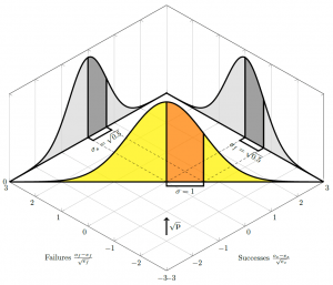
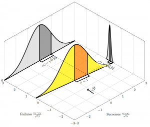
That is, to see that we have unit variance, we need to rotate our perspective to look along the direction of the vector \sqrt{\mathbf{p}}, as illustrated in the figure below (which shows the distribution for a binomial with probability of success p_1=0.5). Looking along the axes, for example, if we consider only the number of successes in the binomial case, and ignore the number of fails, we do have the wrong variance — but that is because we are looking at our distribution from the wrong angle. Aligning ourselves to look at 45 degrees (in this case, since p(\mathrm{success})=0.5 and \sqrt{\mathbf{p}}=\begin{pmatrix}\sqrt{.5}\\\sqrt{.5}\end{pmatrix}), we are suddenly looking at a normal distribution with unit variance.

chi square diagram 2 p=0.5 with root p arrow

If you’re struggling to follow the technical lingo, think of the above diagrams this way. The total number of trials is fixed, so every extra success means one fewer fail. That is why our distribution cuts across the middle of the graph in a straight line; we can’t go anywhere but that line; gaining a success must lose us a fail. If we look at just the successes or the fails in isolation, we have a variance of (1-p_i), just as I was pondering at the top. But when we rotate ourselves to look at this line we are tracing between the two, we can see, just by a simple application of Pythagoras, that our two “wrong” normal distributions collapse into a single normal distribution that has variance of 1. Once we have normal distributions with unit variance, we can compare them against a \chi^2 distribution.

Changing the probability of success

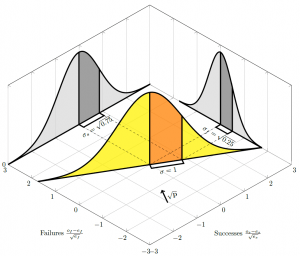
As the probability of success decreases, \sqrt{\mathbf{p}} rotates, and the proportion of variance contributed by each axis changes:

chi square diagram 2 p=0.25 with root p arrow

As p(\mathrm{success}) gets closer and closer to zero, we get closer and closer to a Poisson, and (in this special case) the “Poisson” argument looks more credible; this can be seen as \sqrt{\mathbf{p}} starts to align with the “failures” axis as p(\mathrm{success}) \rightarrow 0 and the variance on the successes axis heads towards unity:

chi square diagram 2 p=0.01 with root p arrow

A Concise Derivation of the Chi-Squared Tests

On this page, I will derive the covariance matrix for the terms \frac{o_i-e_i}{\sqrt{e_i}} in a Chi-Squared Goodness-of-Fit test. It is not necessarily necessary to digest this whole derivation to understand why Chi-Squared tests work; the main point of interest in this post is the final result. For a discussion of this result that avoids the derivation, but tries to build intuitions and visualizations instead, see my other post here.

Preamble/Moan

I wrote this post (in fact, created this blog) out of a frustration with the quality of materials on this topic on the web. Many derivations out there are outright wrong, or gloss over the most important facts. This page, for example, claims that we are using E as the denominator in \frac{(O-E)^2}{E} because E is the variance of a Poisson distribution. But, in general, we do not have a Poisson distribution; if the probability p of a success on any given trial is nontrivial, then the variance is different (often, very different) from this — by a factor of (1-p). They also cannot account for why we lose any degrees of freedom. This page recognises that the (apparent!) error of (1-p) does exist, but wafts it away by saying “There are theoretical reasons, beyond the scope of this book, that make it preferable to omit the factors (1 – pi)”. Seriously?!?! Why would it be preferable to omit a factor that could be arbitrarily far from 1?? And according to that derivation, we still haven’t lost any degrees of freedom anywhere.

Then I found this page and started to realise that the reason there aren’t clear explanations, is because the real explanation is quite complicated, and those other pages I referenced were trying to avoid falling down the hole of trying to make sense of it! That page is absolutely correct, but quite terse, and takes some reading. Finally, I stumbled across this wonderful, clear, derivation. Finally, the penny dropped!

However, looking over the derivation, I felt that it would be possible to capture the underlying gist in far less space, using a little bit of linear algebra. So, what follows is my as-concise-as-possible derivation of the why the Chi-Squared test works. If any of it does not make sense to you, I refer you to the very clear derivation linked at the end of the last paragraph, and on which this was based.

The Derivation

To make this clean, we will need to use vector notation, I’ll define \mathbf{o} to be the vector of m observed counts for each multinomial category, and \mathbf{e} to be the vector of expected values. In the goodness-of-fit test, we are modelling that the observed values are the counts from a multinomial distribution. So \mathbb{E}(\mathbf{o}) = \mathbf{e}, and the observed and expected values will sum to the same value (\mathbf{o}^T\mathbf{1} = \mathbf{e}^T\mathbf{1}).

Our main obstacle is that of finding \mathbb{E}(\mathbf{oo}^T). For this part, I will use the analogy and (similar notation) from the derivation here. Our multinomial is like throwing n balls X_1,…,X_n into m buckets B_1,…,B_m, and our observed values o_i are given by the number of balls in each given bucket:

o_i = \sum_{l=1}^n I(X_l \in B_i).

We can use this analogy to find \mathbb{E}(\mathbf{oo}^T):

\mathbb{E}(o_io_j) = \mathbb{E}\left(\left[\sum\limits_{l=1}^n I(X_l \in B_i)\right]\left[\sum\limits_{l'=1}^n I(X_{l'} \in B_j)\right]\right) = \mathbb{E}\left(\sum_{l,l'} I(X_l \in B_i)I(X_{l'} \in B_j)\right) = \mathbb{E}\left(\sum_{l=l'} I(X_l \in B_i)I(X_{l'} \in B_j) + \sum_{l \neq l'} I(X_l \in B_i)I(X_{l'} \in B_j)\right) = \sum_{l=l'} \underbrace{\mathbb{E}\left(I(X_l \in B_i)I(X_{l'} \in B_j)\right)}_{=I(i=j)p_i} + \sum_{l \neq l'} \underbrace{\mathbb{E}\left(I(X_l \in B_i)I(X_{l'} \in B_j)\right)}_{=p_ip_j} = n \left[ I(i=j)p_i \right] + n(n-1) \left[ p_ip_j \right]

= I(i=j)e_i + \frac{n-1}{n}e_ie_j,

where the result in the first underbrace above comes from the fact that a ball cannot be in two different buckets at the same time (so the \mathbb{E} there is zero for i \neq j).

From this we have:

\mathbb{E}(\mathbf{oo}^T) = \mathrm{diag}(\mathbf{e})+\frac{n-1}{n}\mathbf{ee}^T,

where I have used \mathrm{diag} to denote the placing of the elements of the vector onto the diagonal of an otherwise zero matrix.

From here, deriving the covariance matrix of \mathbf{o}-\mathbf{e} is pretty easy. Making use of the facts that \mathbb{E}(\mathbf{o})=\mathbf{e} and, therefore \mathbb{E}(\mathbf{o}-\mathbf{e})=\mathbf{0}:

\mathrm{cov}(\mathbf{o}-\mathbf{e})
= \mathbb{E}(\mathbf{o}-\mathbf{e})(\mathbf{o}-\mathbf{e})^T
= \mathbb{E}(\mathbf{oo}^T) - \mathbb{E}(\mathbf{o})\mathbf{e}^T - \mathbf{e}\mathbb{E}(\mathbf{o})^T + \mathbf{ee}^T
= \mathbb{E}(\mathbf{oo}^T) - \mathbf{ee}^T
= \left[ \mathrm{diag}(\mathbf{e}) + \frac{n-1}{n}\mathbf{ee}^T \right] - \mathbf{ee}^T
= \mathrm{diag}(\mathbf{e}) -\frac{1}{n}\mathbf{ee}^T

Now, in the chi-squared formula, for each cell, we are calculating \left( \frac{o_i-e_i}{\sqrt{e_i}} \right)^2. What happens when we divide by \sqrt{e_i}? Here, for succinctness, I will use the slight abuse of notation that \sqrt{\mathbf{e}} is calculated by taking the square root of each element of \mathbf{e} independently:

\mathrm{cov} \left(  \left[\mathrm{diag}(\sqrt{\mathbf{e}})\right]^{-1} (\mathbf{o}-\mathbf{e})  \right)
= \left[\mathrm{diag}(\sqrt{\mathbf{e}})\right]^{-1} \mathrm{cov} (\mathbf{o}-\mathbf{e}) \left[\mathrm{diag}(\sqrt{\mathbf{e}}) \right]^{-1}
= \left[\mathrm{diag}(\sqrt{\mathbf{e}})\right]^{-1} \left( \mathrm{diag}(\mathbf{e}) -\frac{1}{n}\mathbf{ee}^T \right) \left[\mathrm{diag}(\sqrt{\mathbf{e}}) \right]^{-1}
= I - \frac{1}{n}\sqrt{\mathbf{e}}\sqrt{\mathbf{e}}^T
= I - \sqrt{\mathbf{p}}\sqrt{\mathbf{p}}^T

where the vector \sqrt{\mathbf{p}} is the vector of the square roots of the probability of each multinomial outcome. Importantly, this vector is a unit vector, so that the covariance matrix is singular, having a zero eigenvalue in the direction \sqrt{\mathbf{p}}, and unit eigenvalues in (m-1) directions orthogonal to it. So, our covariance matrix tells us that our \frac{o_i-e_i}{\sqrt{e_i}} terms are distributed according to a unit sphere that has been squashed flat in on dimension. Looking along the diagonal, we see that each variance in isolation is indeed (1-p_i); it is when we consider the shape of all the terms together that the \chi^2-distributed nature emerges. I go into more intuitions, and present some visualizations, based on this, here.