One thing that always puzzled me, when I first started learning statistics, was the Chi-squared tests. Adding up rescaled squared differences of course gives us a distance measure, but why would the denominator be  ? After all, the variance of a binomial, for example, would be
 = E(1-p)") ,
,
so for this to be Chi-squared distributed, should we not be dividing by ") ? And, if so, is our
? And, if so, is our  statistic not out by a factor of
 ") ? Which, for any reasonable-sized
? Which, for any reasonable-sized  , could be quite a huge discrepancy.
The web turned out to be full of nasty red herrings trying to fool me into the wrong conclusion. I trawled through pages that claim we have a Poisson distributon when we don’t (and which have no way of justifying the degrees of freedom we are using), and pages that admit that their derivations are out by but simply suggest that it’s “preferable to omit the factors (1 – pi) in the denominators” (!).
It’s all in the covariance matrix
Eventually, I found some good resources, and the way it works is really surprisingly nifty! I have detailed some good and bad derivations, along with my own more concise version of the good derivations here, but all you really need to know is that the covariance matrix of your  terms looks like this:
 ,
,
where elements of the (notation-abusing) vector  are the square roots of the probabilities
  of each respective outcome in the multinomial model that we are modelling. I should, of course, stress that the goodness-of-fit test is a model designed for testing multinomial outcomes, and should not be confused with other countable outcomes, for which similar, but subtly different tests can sometimes be derived. Crucially, note that
  is a unit vector (since the probabilities must all sum to one).
What does this covariance matrix tell me?
If you’re super happy with linear algebra and covariance matrices, you can skip to the next subsection. If you’re new to linear algebra (the vectors and matrices I’ve used above), I’ll show you a diagram of it in a minute, and underneath the first diagram is a simpler summary. If you have studied some basic linear algebra, but are not sure how to understand this matrix, think of it this way.
This matrix tells us how much variance we have in any given direction; to find out how much variance we have in a given direction, try multiplying a vector that points in that direction, and see how it gets stretched. For example, if I multiply the vector into this matrix, I will get a vector full of zeros as a result (bear in mind that is a unit vector, so  ). So, we can see that in the direction , our vector gets multiplied by zero, and there is zero variance.
Now, imagine we multiplied a new vector  into this matrix that is orthogonal to (that is,
  ). Then the second term in the covariance matrix will give us zeros, and the matrix acts like the identity matrix: that is, our vector gets stretched by a factor of
  (i.e. not at all!). And the variance in every direction that is orthogonal to is . Furthermore, since it acts as the identity matrix in these orthogonal directions, there is no correlation in the distributions along these vectors.
So, why is this Chi-squared distributed?
So, our covariance matrix explains everything!! If our count table has  elements, then we have one direction () that has zero variance (effectively does not exist), and
 ") orthogonal directions in which we have the variance we wanted of , and zero covariance with each other. To visualize this, we have a unit sphere that has been squashed flat in the direction . When we add up our correlated, non-unit-variance, squared distances
orthogonal directions in which we have the variance we wanted of , and zero covariance with each other. To visualize this, we have a unit sphere that has been squashed flat in the direction . When we add up our correlated, non-unit-variance, squared distances ^2}{e_i}") , we end up with the same squared distance as if we had added up the uncorrelated, unit-variance squared distances orthogonal to .
, we end up with the same squared distance as if we had added up the uncorrelated, unit-variance squared distances orthogonal to .
Assuming that this distribution tends towards being multivariate normal (and central limit theorem gives us that it does), then this squared distance will be }") -distributed (based on the rotational symmetry of the normal distribution).
-distributed (based on the rotational symmetry of the normal distribution).
Visualising the covariance matrix
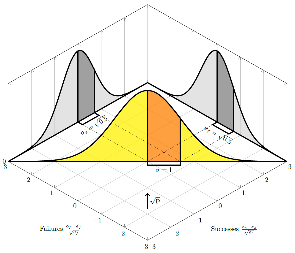
That is, to see that we have unit variance, we need to rotate our perspective to look along the direction of the vector , as illustrated in the figure below (which shows the distribution for a binomial with probability of success  ). Looking along the axes, for example, if we consider only the number of successes in the binomial case, and ignore the number of fails, we do have the wrong variance — but that is because we are looking at our distribution from the wrong angle. Aligning ourselves to look at 45 degrees (in this case, since
 =0.5") and
and  ), we are suddenly looking at a normal distribution with unit variance.

If you’re struggling to follow the technical lingo, think of the above diagrams this way. The total number of trials is fixed, so every extra success means one fewer fail. That is why our distribution cuts across the middle of the graph in a straight line; we can’t go anywhere but that line; gaining a success must lose us a fail. If we look at just the successes or the fails in isolation, we have a variance of ") , just as I was pondering at the top. But when we rotate ourselves to look at this line we are tracing between the two, we can see, just by a simple application of Pythagoras, that our two “wrong” normal distributions collapse into a single normal distribution that has variance of . Once we have normal distributions with unit variance, we can compare them against a distribution.
, just as I was pondering at the top. But when we rotate ourselves to look at this line we are tracing between the two, we can see, just by a simple application of Pythagoras, that our two “wrong” normal distributions collapse into a single normal distribution that has variance of . Once we have normal distributions with unit variance, we can compare them against a distribution.
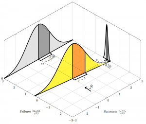
Changing the probability of success
As the probability of success decreases, rotates, and the proportion of variance contributed by each axis changes:
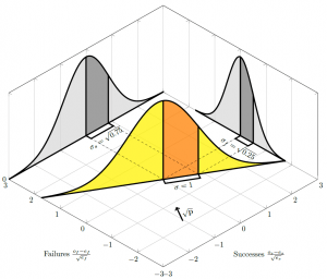
As ") gets closer and closer to zero, we get closer and closer to a Poisson, and (in this special case) the “Poisson” argument looks more credible; this can be seen as starts to align with the “failures” axis as
gets closer and closer to zero, we get closer and closer to a Poisson, and (in this special case) the “Poisson” argument looks more credible; this can be seen as starts to align with the “failures” axis as  \rightarrow 0") and the variance on the successes axis heads towards unity:
and the variance on the successes axis heads towards unity:
Related